David N. Jamieson PhD.
School of Physics
University of Melbourne

Introduction: Magnetism and the forces of nature

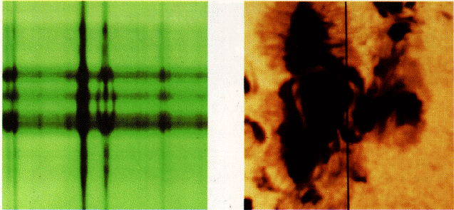
In March 1989, massive magnetic storms on the sun triggered by unusual sunspot activity caused power blackouts in Quebec, Canada, which affected over six million people.

A Met train driver closes a switch causing electric currents to flow into two coils of wire, one firmly anchored to the chassis of the train, the other fixed to the wheels. Powerful magnetic twisting forces propel several hundred tonnes of steel and people down the line.

On the Melbourne Nuclear Microprobe, a special electromagnet, that generates a complicated pattern of magnetic fields, causes a charged particle beam to converge to a tiny point a millionth of a metre in diameter. This is used as a powerful diagnostic probe in medicine, botany, geology and materials science.

A bushwalker, equipped with a magnetic compass, is able to confidently navigate through trackless wilderness by following the Earth's magnetic field.

A hyper-sensitive magnetic field sensor, called a Superconducting Quantum Interference Device, tunes in to the weak magnetic fields generated by thoughts running around nerve paths in human brains.

Magnetic forces are ubiquitous in the natural world and have a prolific range of applications in our technological civilization. Yet there is something troubling about magnetism. As an undergraduate studying Physics, I was worried that magnetic forces were only felt by moving charged particles. This can be seen from the fundamental formula for the force, F, on a particle with charge q moving with velocity v through a region of magnetic and electric fields:

where E and B are the strengths of the electric and magnetic fields. This force is called the Lorentz force. The force from the electric field (the qE bit) seems straight forward enough, but surely the size of the magnetic force (the qv´B bit) depends on who measures it? This is because my measurement of the velocity of the particle will depend on how fast I am going relative to the particle! That is, the velocity of my own personal reference frame relative to the particle. Surely the choice of reference frame should not affect the magnetic force? Indeed, what happens to the magnetic force in the reference frame of the particle itself where the velocity is zero? Is the magnetic force also zero? If this seeming paradox is not enough, many of the formulae for magnetism are amazingly similar to equivalent formulae that apply to electrostatic forces, but have some suggestive asymmetries. More on this later.

It is the aim of this essay to highlight some of the things that set magnetism apart from the other forces, then explain why this should be so.

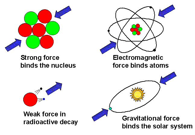
Let us review the different types of force and see where magnetism fits in. There are four forces in nature (recent suggestions that there may be a "fifth force" have not been proven by experiment). These are, starting with the most familiar:

• Gravity. This is the force that gives us up and down, most of us (apart from a few astro- and cosmo-nauts) spend all our lives immersed in the gravitational field of the Earth.
• Electromagnetism. This lumps electrostatic and magnetic forces together, for reasons that I hope will become clear at the end of this lecture. Most people will be familiar with electrostatic forces from the way a piece of plastic (in ancient times a piece of amber), when rubbed with a piece of fabric, will pick up small pieces of paper. Electrostatic forces also keep us from falling through the floor! It is the repulsion between surface electrons that prevent two objects from occupying the same place. Some familiar instances of the magnetic force have been described already.
• The Strong Nuclear Force. This is the force that binds neutrons and protons together in the nucleus of atoms. It acts only over a short range but is significantly more powerful than the electrostatic force that would otherwise cause the positively charged protons to violently repel each other. The average person doesn't experience this force directly, but I see ample evidence for it when I bombard light elements, like carbon, with fast protons as part of my research activities. The interaction between the proton and the carbon nucleus is dramatically affected by the strong force.
• The Weak Nuclear Force. This force is involved, amongst other things, in certain types of radioactive decay. Our own bodies contain readily measurable amounts of a radioactive isotope of potassium that is quietly decaying away because of the action of the weak nuclear force.

The History of Magnetism

Ca. 1000 BC: According to the classical Greek historian Pliny, the word magnetism derives from the name of a shepherd boy called Magnes, who finds that his iron tipped staff is attracted to lumps of naturally occurring magnetite (magnetic iron oxide) on Mt Ida, Greece. Around the same time, Chinese navigators discover that a lump of lodestone (another name for magnetite) suspended on a thread always points in the same direction. The story about the shepherd boy is probably more legendary than historical, but during the next 3000 years, the study of magnetism is confined to naturally occurring permanent magnets.

1269: Pierre Pelèrin de Maricourt discovers that a spherical lodestone has two places on the surface where lines of magnetic force converge. He calls them "poles" by analogy with those of the Earth.

Study of naturally occurring permanent magnets reveals several more important properties. It is found that breaking a magnet in half always results in two new magnets each with its own North and South poles. It is never possible to produce a magnet that has just a North or just a South pole. This is quite unlike the behaviour of charged objects, where it is readily possible to give an object either a positive or a negative charge. Permanent magnets always appear as dipoles. This is another clue that there is something unusual about magnetism.

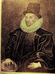
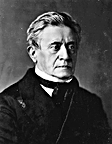
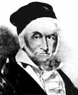
1600: To explain how a compass works, William Gilbert (1540-1603)i postulates that the Earth acts like a huge spherical magnet with North and South poles. Gilbert is also credited with being the first to use the terms "electric force" and "electricity", which derive from the Greek word for "amber".

1820: While setting up a lecture demonstration for a physics class a Danish Physics Lecturer, Hans Christian Oersted (1777-1851), notices that an electric current in a wire deflects a compass needle. The electric current was producing a magnetic field! The science of "electromagnetism" is founded.

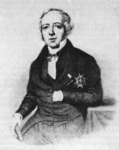
1821: Andre Marie Ampére (1775-1836) determines the law, which now bears his name, for the relationship between the current flowing in a wire and the magnetic field it generates.

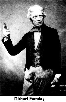
1831: Michael Faraday (1791-1867) and, independently, Joseph Henry (1797-1878) show how a changing magnetic field threading a loop of wire can induce an electric current in the loop. Faraday is the first to publish, so the theory for the result is now called "Faraday"s law of induction". Most electric power is generated by exploiting Faraday"s law.

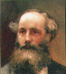
1873: James Clerk Maxwell (1831-1879) publishes his "Treatise on Electricity and Magnetism" containing a comprehensive theory of all the discoveries so far. However it is the lone British eccentric Oliver Heaviside (1850-1925) who distils the essence of the theory from Maxwell"s vastly complicated mathematics into the elegantly simple form we know today as the Maxwell equations.

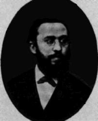
1895: Hendrik Lorentz (1853-1944) decides that the Maxwell equations can be understood at a fundamental level as the interaction of moving charged particles. It is not until 1899 that these moving charged particles become known as electrons. Lorentz introduces the formula for the force experienced by a charged particle moving in electric and magnetic fields that we now call the Lorentz force, discussed earlier.

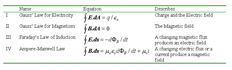Figure Figure 4: The Maxwell equations.

Although the Maxwell equations are remarkably symmetrical between the roles of the electric and magnetic fields, there are some glaring asymmetries. These asymmetries are due to the lack of a magnetic equivalent of the electron: the magnetic monopole. For example Gauss’s law for magnetism denies a role for magnetic monopoles in the origin of a magnetic field. This is in agreement with experiment, because magnetic monopoles have never been found, despite exhaustive searching. Also, Faraday’s law contains no term for "monopole currents" which would be analogous to the term for electric current in the Ampere-Maxwell law.

The Maxwell equations tell us how magnetic fields are generated, either by electric currents, or changing electric fields. The Lorentz force formula tells us how magnetic fields affect moving charged particles. Yet how is it that permanent magnets can generate magnetic fields, apparently without electric currents, and feel the effect of magnetic forces, apparently without containing moving charged particles? The answer is that they do indeed contain moving charged particles! Another result from the late nineteenth century is needed:

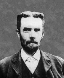
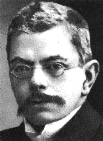
1896: Pieter Zeeman (1865-1943) discovers the effect, for which he would share the 1902 Nobel prize with Lorentz, that spectral lines would broaden if the source is placed in a magnetic field. Experiments in 1897 show actual splitting of the lines. These results are interpreted as the effect of the Lorentz force on moving electrons inside atoms. We know now that electrons in atoms jumping between energy levels produce spectral lines, so any affect on the way they move shows up in a shift of the lines.

Today we regard the spinning electrons inside atoms as existing as quantum mechanical standing waves. Despite this, the electrons still act like tiny loops of current running around the atom. The Maxwell equations tell us that this loop of current will generate a magnetic field. In most atoms, the magnetic fields generated by all these tiny current loops cancel out. But in iron and some other ferromagnetic materials, they do not, each atom acts like a tiny magnet. Under favourable circumstances, many of these tiny atomic magnets are locked into alignment and hence we have a permanent magnet. The aligned atomic magnets can then reach out and temporarily align the tiny magnets in lumps of unmagnetised iron, and attract them. Also, they can attract or repel other magnets depending on whether opposite or alike poles are together. The superimposed effect of all the aligned spinning electrons in a ferromagnetic material is called a "lattice current".

So we see that in both permanent magnets and electromagnets, movement of charged particles, usually currents of electrons, is essential to generate magnetic forces, and in turn, movement of charged particles is essential to "feel" magnetic forces.

There was an abundance of restlessly moving charged particles in the examples of magnetism at the start of this essay. Currents of fusion plasma around sunspots in the sun generate the magnetic fields which then disturbed the currents in the Canadian electricity grid. Electric currents in the field windings of train motors produce magnetic fields which act on the currents in the armature windings, forcing them to rotate. The currents in the windings of the special electromagnets on the Melbourne Nuclear Microprobe produce magnetic fields which force a broad charged particle beam to converge to a fine probe. In the Earth, "magnetohydrodynamic" currents in the core generate the Earth’s magnetic field (by a mechanism that is not yet fully understood) which then acts on the lattice currents in the magnetised compass needle forcing it to point north. In the human brain, weak electric currents running through nerves generate magnetic fields that can be detected by subtle effects on peculiar supercurrents of electron pairs in a superconductor.

So at last in our history of magnetism we come to the golden year for physics:

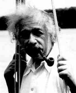
1905: Albert Einstein (1879-1955) publishes his paper "Electrodynamics of Moving Bodies" which contains the Special Theory of Relativity. Einstein was later to remark about this paper:

"What led me more or less directly to the Special Theory of Relativity was the conviction that the electromotive force acting on a body in motion in a magnetic field was nothing else but an electric field."

A. Einstein (1952), from a letter to the Michelson Commemorative Meeting of the Cleveland Physics Society, quoted by R.S. Shankland, Am. J. Phys., 32, 16 (1964), p35.

What does Einstein mean by this? Let us look closely at an example.

Let us take a close look at what happens when a moving charged particle is deflected by the magnetic force generated by a current in a piece of metal wire. First of all, a piece of wire by itself is electrically neutral. The outermost electron in a metal is free to move about, so we can think of the wire as a fixed array of positive metal ions surrounded by a sea of free electrons. For simplicity, we will assume that each metal atom contributes only one free electron to the sea. A nearby charged particle, taken for example to carry a positive charge, does not feel any force from the neutral wire, since the attractive force from the electrons cancels out the repulsive force from the metal ions. When an electric current is switched on, the free electrons begin to flow through the wire.

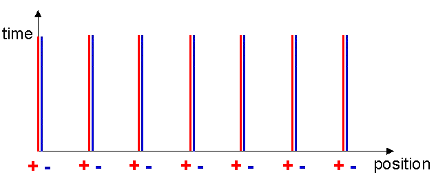
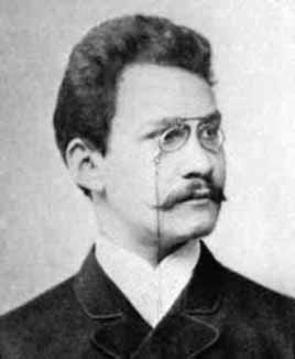
As a useful technique of visualising what is going on, let me introduce the concept of the Minkowski diagram. These diagrams are named after Hurwitz Minkowski (1864-1909) who taught the young Einstein at the Zurich Polytechnic in 1896, but was later to make significant contributions to the mathematics of the theory of relativity. A Minkowski diagram is like a map that provides an overview of how objects move through time and space. For example, figure 6 represents the situation for our wire with no current in it. Both the metal ions and the free electrons are stationary, hence always stay at the same x-coordinate. (I am neglecting thermal effects that only cause the ions and free electrons to move randomly about some mean position.) Vertical lines representing their position as a function of time may therefore represent the positions. These are called world lines. As time passes, the x-coordinates do not change.

Consider now the effect of switching on an electric current. The electrons begin to move along the wire with a uniform velocity, v. Of course in a real wire the electrons are constantly accelerating and scattering off the metal ions, but the overall effect is for a uniform drift through the wire propelled by the applied voltage that overcomes the resistance of the wire.

We can write:

where v is the drift velocity of the electrons, i is the current in the wire, e is the charge on an electron, A is the cross sectional area of the wire and N_e is the number of electrons per unit volume. We can also introduce a quantity which will be useful later called the linear charge density, l_-:

The linear charge density is just the amount of free electron charge per metre along the wire. This will be a negative number since the electrons carry a negative charge, however, since we have assumed each metal atom contributes one electron this will be balanced by the equal and opposite positive charge density from the metal ions, l₊:

We know by experiment that a current carrying wire generates a magnetic field that exerts a magnetic force on moving charged particles, but not on stationary charged particles. Let us try to understand the origin of this magnetic force by looking at the situation from the point of view of the moving charge. To make everything nice and simple we will assume the moving charge has a velocity v in the same direction as the moving electrons in the wire. This would be the situation if the moving charge were moving in a current in a second wire.

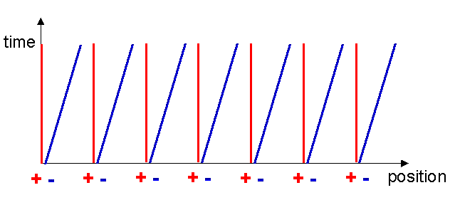
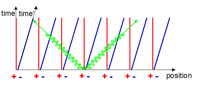
Let us construct the Minkowski diagram for the current carrying wire. The world lines of the metal ions remain the same as before since they are not moving, however the electron world lines become inclined to the x-axis since the x-coordinates of the electrons are increasing with time (see figure 7). At a time t₁ after the current was switched on, the x-coordinate of an electron has increased by an amount vt₁.

 

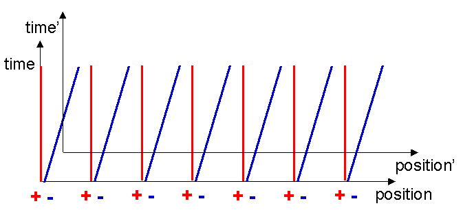
We can now mark on this diagram the reference frame of a nearby stationary charged particle. A reference frame is simply a device we carry around to help us perceive the outside world. Perception of the outside world involves measuring distances and times of things going on around us. We can simply draw in the reference frame of the stationary particle with its x’ and t’ axes parallel to the x and t axes, see figure 8. Notice that in the new frame the separation between the positive metal ions and the moving negative free electrons is just the same as before. This can be understood by careful consideration of the effect on the electrons of the acceleration they experience when the current is switched on. Since the spacing of the electrons has not changed, the positive and negative linear charge densities again have the same magnitude so the attractive and repulsive forces cancel each other out and the stationary charged particle feels no electrostatic force:

We already know that despite the fact that a current of electrons produces a magnetic field, the stationary charged particle does not feel a magnetic force. The Lorentz force formula tells us that the magnetic force is zero if the velocity is zero.

 

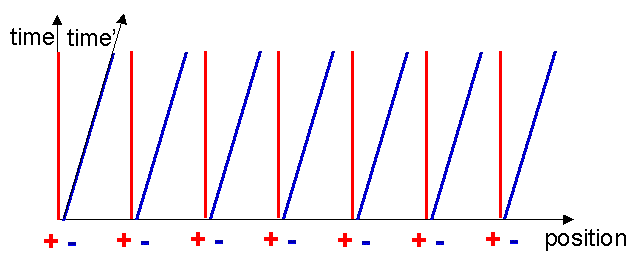
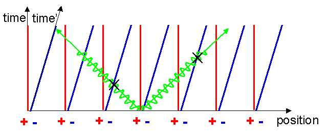
Consider a nearby moving charged particle. In this case the Lorentz force formula tells us that such a moving particle will feel a magnetic force equal to qv´ B. Let us now look at the situation from the point of view of the moving charged particle. In its own reference frame, it is stationary, v=0, therefore it cannot feel any magnetic forces which depend only on velocity. Is it possible it feels some other sort of force? It will be helpful in our check of this if we mark in on our Minkowski diagram the reference frame of the moving particle. What does its reference frame look like? Well, a point stationary on the origin of the moving particle’s reference frame can be represented by a line like those for the electrons. I will assume that the moving particle was located at the origin of the original frame when the current was switched on. The world line of the origin of the moving frame also represents the t’-axis of the moving frame, by definition (see figure 9).

Drawing the x’-axis is a bit more difficult. Remember that the x’-axis simply delineates the string of simultaneous events which occurred at t’=0. If we can find two events that are simultaneous in the moving frame, we can find the x’-axis. To do this, assume that one of the electrons somehow emits a flash of light at t=0 as shown in figure 10.

We can define two simultaneous events in the moving frame as the events represented by the receipt of this flash by the two equidistant adjoining electrons. These are marked with two crosses in figure 11.  Remember that the electrons don’t know they are moving, they see that the positive metal ions are moving backwards past them.

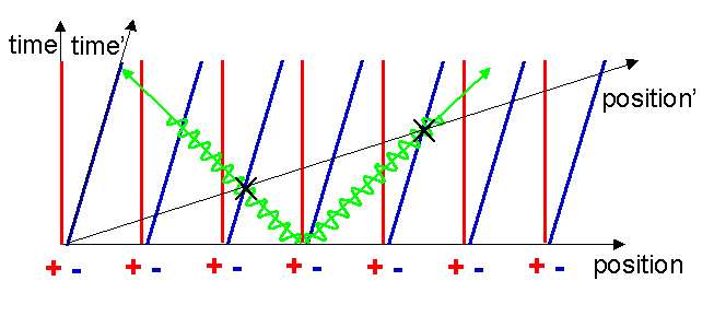
Now we need an extraordinary extra piece of physics to see what happens next. One of the most amazing things about the way the universe works is that the speed of light is the same for all observers. No matter how fast you go, the speed of light always stays the same! This was the main insight of Einstein in 1905 and is the foundation on which all of optics and electromagnetism rests.

The speed of light is the same in all reference frames, independent of the speed of the source. Now, since the electrons are equidistantly spaced along the x’-axis, receipt of the light flashes represent simultaneous events in their moving reference frame. Hence the x’-axis is just a line through the two crosses, starting at the common origin. Notice that events marked by the two crosses are not simultaneous in the original reference frame.

 

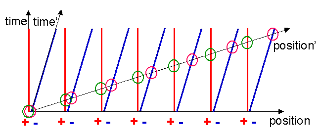
Notice now a startling thing, the electron world lines cut the x’-axis with a wider spacing compared to the metal ion world lines! These points are marked with the green and pink circles in figure 13.  In the reference frame of the moving charge, the charge density of the electrons is less than that of the metal ions! We now have:

Hence the attractive and repulsive forces are no longer balanced, which results in a net electrostatic force acting on the charged particle.

If we carefully do the algebra required to transform this electrostatic force back into the original reference frame of the metal ions, in which the nearby charged particle is moving, we find that it is equal to the magnetic force that we expect to find! In other words, what the moving charged particle experiences as a purely electrostatic force from the unbalanced linear charge densities is described in the original reference frame as a velocity dependent force, which is what we call a magnetic force.

The imbalance in the linear charge densities between the positive metal ions and the moving electrons, measured in the reference frame of the moving charge, is a result of the Lorentz contraction due to the relative motions of the nearby charged particle, the electrons flowing in the wire and the metal ions. This relativistic effect is perhaps most familiar to us when applied to fast moving objects. Let us see how fast the electrons are moving in a typical current carrying wire. In a copper wire the density of copper atoms is about 8.5´10²² atoms per cubic centimetre, and hence the density of free electrons is about the same. In a copper wire with a cross sectional area of 1 square millimetre and carrying a current of 10 Amps the formula for v given above shows that the electron velocity is only 0.7 millimetres per second. This is an extremely small velocity! The Lorentz contraction for such a small velocity differs from 1 by only 3´10^-24. This unimaginably small contraction is nevertheless sufficient to cause a slight imbalance in the positive and negative charge densities of the wire that causes moving charged particles to feel a magnetic force.

Keep it in mind that this magnetic force is tremendously weaker than either of the two, almost balanced, electrostatic forces from the electrons or the metal ions. If the free electrons from 1 metre of wire could be fully separated by 10 centimetres from the positive metal ions then the attractive electrostatic forces between these two lumps of negative and positive charges would be about equal to the gravitational force between the Earth and the Moon! It is the enormous strength of the electrostatic forces that is the reason why we don’t often use them directly in our technological applications. It is simply too hard to separate positive and negative charges. It is much easier to exploit the incredibly slight imbalance brought about by the relativistic Lorentz contraction that is noticeable as magnetism.

Think about that next time you feel the mysterious tug of a magnet.